%load_ext autoreload
%autoreload 2
import numpy as np
import pandas as pd
import seaborn as sns
from matplotlib import pyplot as plt
np.seterr(all='ignore')

from sklearn.datasets import make_blobsHere is the link to my source code (source.py):
https://github.com/Sallyliubj/Sallyliubj.github.io/blob/main/posts/LogisticRegression%20/source.py
Objective:
This blog consists of four parts:
The implementation and testing of regular Logistic Regression Model.
The implementation ans testing of Stochastic Logistic Regression Model.
The adding of momentum to my Stochastic Logistic Regression Model.
The experimentation with the three methods, including three cases discussing how the learning rate, batch size, and momentum would affect the convergence of Logistic Regression.
Generate a random data set:
First, I generate a set of data, shown as below.
np.random.seed(123)
p_features = 3
X, y = make_blobs(n_samples = 200, n_features = p_features - 1, centers = [(-1, -1), (1, 1)])

fig = plt.scatter(X[:,0], X[:,1], c = y)
xlab = plt.xlabel("Feature 1")
ylab = plt.ylabel("Feature 2")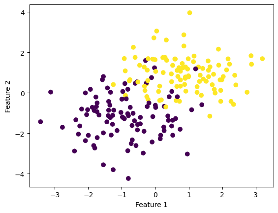
Part 1. Logistic Regression Algorithm
I implement my simple logistic regression model to fit the data:
from source import LogisticRegression

LR = LogisticRegression()
LR.fit(X, y, alpha = 0.05, max_epochs = 1000)
#LR.w
Testing of simple Logistic Regression Method:
I visualize the prediction by drawing a line to separate the data. I also trace the history of logistic loss (empirical risk) to see if it converges at the end.
X_ = LR.pad(X)
loss = LR.loss(X_, y)

fig, axarr = plt.subplots(1, 2)

axarr[0].scatter(X_[:,0], X_[:,1], c = y)
axarr[0].set(xlabel = "Feature 1", ylabel = "Feature 2", title = f"Loss = {loss}")

f1 = np.linspace(-3, 3, 101)

p = axarr[0].plot(f1, (LR.w[2] - f1*LR.w[0])/LR.w[1], color = "black")

axarr[1].plot(LR.loss_history)
axarr[1].set(xlabel = "Iteration number", ylabel = "Loss")
plt.tight_layout()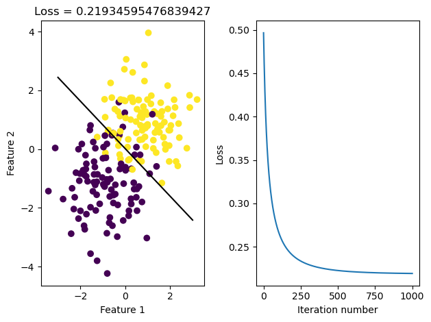
print(LR.score_history[-5:])
#print(LR.loss_history[-5:])
#print(LR.w)
[0.895, 0.895, 0.895, 0.895, 0.895]Based on the graph of loss history shown above, gradient descent seems to be convergent.
Note:
Since the data are not linearly separable, we cannot draw a perfect separating line, and the score (accuracy) will never reach 1.0. In this set of data, the score reaches 0.895 at the end.
Part 2. Stochastic Gradient Descent Method
I implement the Stochastic Gradient Descent Method and fit the data:
LR2 = LogisticRegression()
LR2.fit_stochastic(X, y, alpha = 0.01, max_epochs = 500, batch_size = 15)
Testing of fit_stochastoic method for Logistic Regression:
Similar to what I did above, I visualize the corresponding line, and track the value of the loss achieved:
X_ = LR.pad(X)
loss = LR2.loss(X_, y)

fig, axarr = plt.subplots(1, 2)

axarr[0].scatter(X_[:,0], X_[:,1], c = y)
axarr[0].set(xlabel = "Feature 1", ylabel = "Feature 2", title = f"Loss = {loss}")

f1 = np.linspace(-3, 3, 101)

p = axarr[0].plot(f1, (LR2.w[2] - f1*LR2.w[0])/LR2.w[1], color = "black")

axarr[1].plot(LR2.loss_history)
axarr[1].set(xlabel = "Iteration number", ylabel = "Loss")
plt.tight_layout()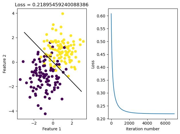
print(LR2.loss_history[-5:])
print(LR.w)
[0.21894443974814265, 0.2189453010824046, 0.21894371455305317, 0.21894288134945547, 0.21894209558615926]
[1.55870232 1.94248526 0.03479441]Based on the graph of the loss history shown above, the stochastic gradient descent seems to be convergent.
Part 3. Momentum
I implement the momentum method for stochastic gradient descent. If the user sets momentum = True then I set the parameter to value 0.8. Otherwise it is set to 0, and we have regular gradient descent.
Here I generate a set of data with 10 feature dimensions.
np.random.seed(123)
p_features = 10
X, y = make_blobs(n_samples = 200, n_features = p_features - 1, centers = [(-1, -1), (1, 1)])
Comparing the three fit methods
Here is a plot showing the evolution of the loss function for the three algorithms:
#Fit and plot the graph for stochastic gradient with momentum
LR3 = LogisticRegression()
LR3.fit_stochastic(X, y,
                  max_epochs = 1000,
                  momentum = True,
                  batch_size = 10,
                  alpha = .1)

num_steps = len(LR3.loss_history)
plt.plot(np.arange(num_steps) + 1, LR3.loss_history, label = "stochastic gradient (momentum)")


#Fit and plot the graph for stochastic gradient without momentum
LR4 = LogisticRegression()
LR4.fit_stochastic(X, y,
                  max_epochs = 1000,
                  momentum = False,
                  batch_size = 10,
                  alpha = .1)

num_steps = len(LR4.loss_history)
plt.plot(np.arange(num_steps) + 1, LR4.loss_history, label = "stochastic gradient")


#Fit and plot the graph for standard  gradient
LR5 = LogisticRegression()
LR5.fit(X, y, alpha = .05, max_epochs = 2000)

num_steps = len(LR5.loss_history)
plt.plot(np.arange(num_steps) + 1, LR5.loss_history, label = "gradient")

plt.xlabel("iteration")
plt.ylabel("loss")
plt.loglog()

legend = plt.legend() 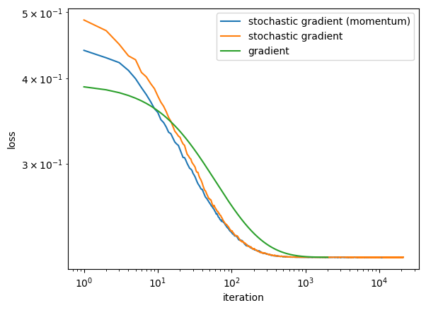
Based on the graph, stochastic gradient descent with and without momentum tends to converge at a rate faster than standard gradient descent, but these random algorithms can “bounce around” near the good solution. Standard gradient descent might need more epochs to find a good solution, but quickly “settles down” once it finds it.
Part 4. Perform Experiments
After testing and implementing my Logistic Regression class, I will now perform experiments to show examples of the following phenomena:
Case 1:
A case in which gradient descent does not converge to a minimizer because the learning rate (alpha) is too large:
#Fit and plot the graph for stochastic gradient with momentum
LR3 = LogisticRegression()
LR3.fit_stochastic(X, y,
                  max_epochs = 1000,
                  momentum = True,
                  batch_size = 10,
                  alpha = .9)

num_steps = len(LR3.loss_history)
plt.plot(np.arange(num_steps) + 1, LR3.loss_history, label = "stochastic gradient (momentum)")


#Fit and plot the graph for stochastic gradient without momentum
LR4 = LogisticRegression()
LR4.fit_stochastic(X, y,
                  max_epochs = 1000,
                  momentum = False,
                  batch_size = 10,
                  alpha = .9)

num_steps = len(LR4.loss_history)
plt.plot(np.arange(num_steps) + 1, LR4.loss_history, label = "stochastic gradient")


#Fit and plot the graph for gradient
LR5 = LogisticRegression()
LR5.fit(X, y, alpha = .9, max_epochs = 1000)

num_steps = len(LR5.loss_history)
plt.plot(np.arange(num_steps) + 1, LR5.loss_history, label = "gradient")

plt.xlabel("iteration")
plt.ylabel("loss")
plt.loglog()

legend = plt.legend() 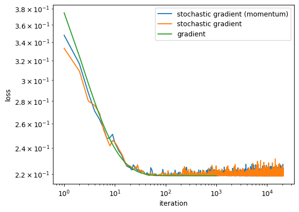
From the graph above, when I set alpha to 0.9, the three lines describing the three algorithms cannot converge to a minimizer.
Case 2:
A case in which the choice of batch size influences how quickly the algorithm converges.
#Fit and plot the graph for stochastic gradient with batch_size = 20
LR3 = LogisticRegression()
LR3.fit_stochastic(X, y,
                  max_epochs = 500,
                  momentum = False,
                  batch_size = 10,
                  alpha = .01)

num_steps = len(LR3.loss_history)
plt.plot(np.arange(num_steps) + 1, LR3.loss_history, label = "stochastic gradient batch_size=10")


#Fit and plot the graph for stochastic gradient with batch_size = 50
LR4 = LogisticRegression()
LR4.fit_stochastic(X, y,
                  max_epochs = 500,
                  momentum = False,
                  batch_size = 30,
                  alpha = .01)

num_steps = len(LR4.loss_history)
plt.plot(np.arange(num_steps) + 1, LR4.loss_history, label = "stochastic gradient batch_size=30")

#Fit and plot the graph for stochastic gradient with batch_size = 90
LR5 = LogisticRegression()
LR5.fit_stochastic(X, y,
                  max_epochs = 500,
                  momentum = False,
                  batch_size = 90,
                  alpha = .01)

num_steps = len(LR5.loss_history)
plt.plot(np.arange(num_steps) + 1, LR5.loss_history, label = "stochastic gradient batch_size=90")

plt.xlabel("iteration")
plt.ylabel("loss")
plt.loglog()
legend = plt.legend() 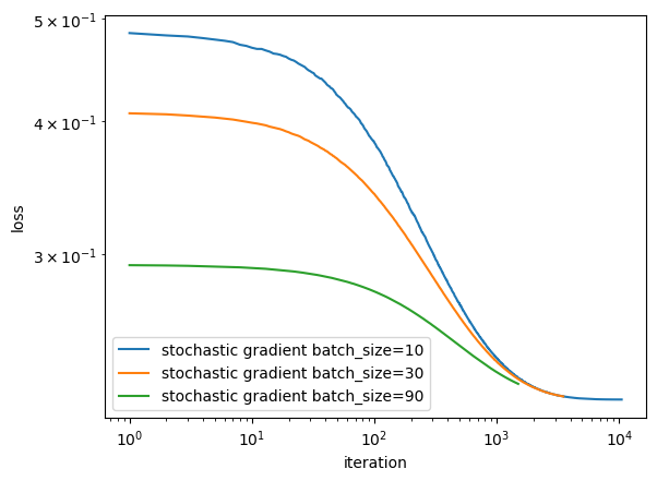
Compare the there lines with different batch size, the green line with batch_size = 90 seems to converge faster then the other two line.
However, by constantly experimentating with different batch sizes, I noticed that it may not always be the same case. Sometimes the line with smaller batch size may converge more quickly.
After trying different batch sizes, I can conclude that on average, the larger batch size tends to converge faster.
Case 3:
A case in which the use of momentum significantly speeds up convergence.
#Fit and plot the graph for stochastic gradient with momentum
LR3 = LogisticRegression()
LR3.fit_stochastic(X, y,
                  max_epochs = 500,
                  momentum = True,
                  batch_size = 40,
                  alpha = .05)

num_steps = len(LR3.loss_history)
plt.plot(np.arange(num_steps) + 1, LR3.loss_history, label = "stochastic gradient (momentum)")


#Fit and plot the graph for stochastic gradient without momentum
LR4 = LogisticRegression()
LR4.fit_stochastic(X, y,
                  max_epochs = 500,
                  momentum = False,
                  batch_size = 40,
                  alpha = .05)

num_steps = len(LR4.loss_history)
plt.plot(np.arange(num_steps) + 1, LR4.loss_history, label = "stochastic gradient")

plt.xlabel("iteration")
plt.ylabel("loss")
plt.loglog()

legend = plt.legend() 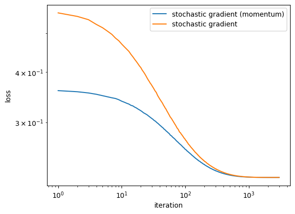
Comparing to the two lines in the graph, the gradient descent with momentum (blue line) tend to converge faster than the other line.
Conclusion:
According to these experimentations, I find that by changing the learning rate, batch size, and momentum, the performance of my Logistic Regression Model differs significantly.
Therefore, it is important to choose the appropriate value of alpha, batch size, and momentum in order for the model to perform the accurate prediction.