%load_ext autoreload
%autoreload 2
import numpy as np
import pandas as pd
import seaborn as sns
from matplotlib import pyplot as plt

import sklearn
from sklearn.datasets import make_blobsHere is the link to my source code (source.py):
https://github.com/Sallyliubj/Sallyliubj.github.io/blob/main/posts/perceptron%20blog%20post/source.py
Objective
This blog post consists of three parts:
The implementation of my percpetron algorithm.
The testing and experimentation of my perceptron algorithm, including three different cases that describe the model’s behavior with different data.
The discussion of the time complexity of my algorithm.
Part 1. Implementation
First, I implement my perceptron algorithm:
from source import Perceptron
p = Perceptron()
Part 2. Experimentation
Next I will experiment with my algorithm to test its performance under different dataset.
I will consider three cases:
A linearly separable data in the 2D space.
A non-linearly separable data in the 2D space.
A dataset in higher dimensions.
Case 1:
I want to show that when the 2d data that is linearly separable, then the perceptron algorithm converges to weight vector describing a separating line (provided that the maximum number of iterations is large enough).
To test this idea, I generated a linarly separable dataset and implemented my perceptron algorithm
np.random.seed(12345)
n = 100
p_features = 3

X, y = make_blobs(n_samples = 100, n_features = p_features - 1, centers = [(-1.7, -1.7), (1.7, 1.7)])

fig = plt.scatter(X[:,0], X[:,1], c = y)
xlab = plt.xlabel("Feature 1")
ylab = plt.ylabel("Feature 2")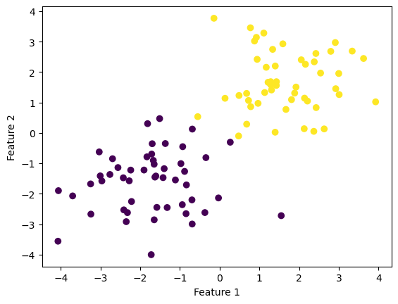
Then I implement my perceptron algorithm and fit the data:
p.fit(X, y, max_steps = 1000)Trace the accuracy:
print(p.history[-10:]) #check the last few values

fig = plt.plot(p.history)
xlab = plt.xlabel("Iteration")
ylab = plt.ylabel("Accuracy")
[0.99, 0.99, 0.99, 0.99, 0.99, 0.99, 0.99, 0.99, 0.99, 1.0]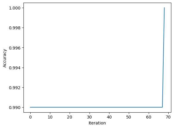
The figure above shows the evolution of the accuracy over traning.
After iterations, the accuracy of the data finally reached 1.0.
Draw the line:
def draw_line(w, x_min, x_max):
  x = np.linspace(x_min, x_max, 101)
  y = -(w[0]*x + w[2])/w[1]
  plt.plot(x, y, color = "black")

fig = plt.scatter(X[:,0], X[:,1], c = y)
fig = draw_line(p.w, -2, 2)

xlab = plt.xlabel("Feature 1")
ylab = plt.ylabel("Feature 2")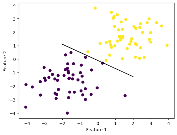
Since the data are linearly separable, I could draw a separating line that separate the data.
Case 2:
For 2d data, when the data is not linearly separable, the perceptron algorithm will not settle on a final value of w, but will instead run until the maximum number of iterations is reached, without achieving perfect accuracy.
To test this idea, I generated a non-linearly separable dataset and visualized it as below.
import numpy as np
from sklearn.datasets import make_circles
#sklearn.datasets.make_circles(n_samples=100, *, shuffle=True, noise=None, random_state=None, factor=0.8)

np.random.seed(4)
numPoints = 20
X, y = make_circles(n_samples=100,
  factor=.8, noise=.05)
X = 10 * X
#for i in range(0, numPoints):
  #print(str(X[i][0]) + ", " +
   #     str(X[i][1]) + ", " +
    #    str(y[i]))


fig = plt.scatter(X[:,0], X[:,1], c = y)
xlab = plt.xlabel("Feature 1")
ylab = plt.ylabel("Feature 2")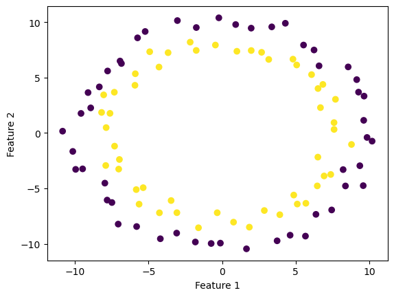
Then I implemented my perceptron algorithm to see its performance.
p.fit(X, y, max_steps = 1000)Trace the accuracy:
fig = plt.plot(p.history)
xlab = plt.xlabel("Iteration")
ylab = plt.ylabel("Accuracy")

print(p.history[-10:]) #check the last few values
[0.49, 0.49, 0.5, 0.5, 0.5, 0.5, 0.49, 0.51, 0.5, 0.51]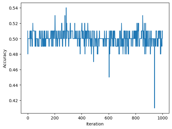
The figure above shows the evolution of the accuracy over traning. After reaching the maximum steps of iterations, the accuracy of the data is still around 0.5, which does not converge to 1.0.
Draw the line:
def draw_line(w, x_min, x_max):
  x = np.linspace(x_min, x_max, 101)
  y = -(w[0]*x + w[2])/w[1]
  plt.plot(x, y, color = "black")

fig = plt.scatter(X[:,0], X[:,1], c = y)
fig = draw_line(p.w, -2, 2)

xlab = plt.xlabel("Feature 1")
ylab = plt.ylabel("Feature 2")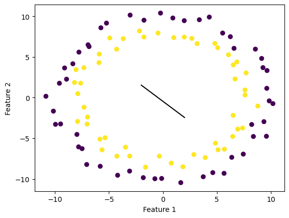
From the line I drew above, it can be seen that the line cannot separate the data at all.
Case 3:
I want to show that my perceptron algorithm is also able to work in more than 2 dimensions. I generate a dataset with p_features = 6.
n = 100
p_features = 6
X, y = make_blobs(n_samples = 100, n_features = p_features - 1, centers = [(-1.7, -1.7), (1.7, 1.7)])
I implemented my perceptron algorithm, which cannot be visualized since it is more than 2d.
p.fit(X, y, max_steps = 1000)Trace the accuracy:
print(p.history[-10:]) #check the last few values

fig = plt.plot(p.history)
xlab = plt.xlabel("Iteration")
ylab = plt.ylabel("Accuracy")
[0.99, 0.99, 0.99, 0.99, 0.99, 0.99, 0.99, 0.99, 0.99, 1.0]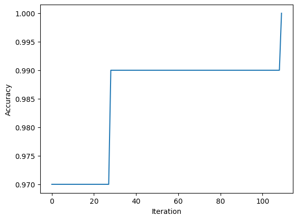
The graph above shows the evolution of the accuracy over traning.
- Since the score eventually reached 1.0, my perceotion algiorithm converges to a weight vector describing a separating line. Therefore, I can conclude that the data is linearly separable.
Part 3. Discussion:
Question:
What is the runtime complexity of a single iteration of the perceptron algorithm update as described by Equation 1?
Assume that the relevant operations are addition and multiplication. Does the runtime complexity depend on the number of data points? What about the number of features?
Answer:
The runtime complexity does not depend on the number of data points, but depends on the number of features.
Explanation:
- X_ has dimension n x p; X_[i] has dimension 1 x p
- y_ and y_predict both has n elements
- w has length p
Run-time Analysis:
First, compute the dot product of two vectors w and X[i] with length p, we have time complexity O(p). The result is a number.
Then, multipy the number by a vector X[i] with length p, we still have time complexity O(p). The result is a vector with length p.
So now we get O(p) + O(p) = O(p)
- Finally, add two vectors with lengths of p together, we have time complexity O(p).
So the time complexity should be O(p) + O(p) + O(p) = O(p). The runtime only depends on the value of p.
Conclusion:
When the number of features p increases, each row of X_ has more elements, resulting in more multiplications. So the runtime will increase.
When the number of data points n increases, it does not affect the runtime of a single perceptron update, since each update only considers one data point i.